Cellular Senescence and Genome Wide Methylation Analysis

Recently we conducted a study into the pattern of methylation within senescent cells.

Senescence

Senescence is the permanent halt of proliferation associated with cellular stresses including DNA damage, damaged or short telomeres and oxidative stress.  Senescence dates back to the Hayflick limit and, while there are no definitive markers, cells typically become large and flat and can be identified by the presence of SA-β-GAL, SAHF and tumour suppression networks (i.e. p53 / p16).

Senescence is thought to be a tumour suppression mechanism, through blocking clonal proliferation of cancer cells, and a promoter of ageing via an inflammaging phenotype.  Cancer cells must somehow bypass senescence in order to continue proliferating.

Methylation 

We were interested in studying genome-wide DNA methylation patterns within senescence.  DNA methylation is the addition of a Methyl group to specific DNA bases.  In mammals this is restricted to the cytosine nucleotide (C) within DNA.  Methylation is largely localised at CpG's (a cytosine nucleotide followed by a guamine nucleotide) within the genome.

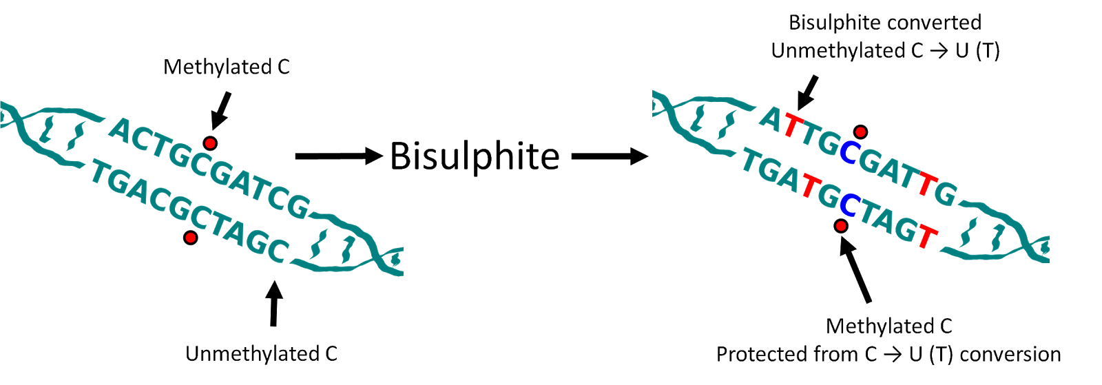
In order to study DNA methylation we use whole genome sequencing combined with bisulphite treatment.  Bisulphite treatment of DNA converts unmethylated cytosines into uracil - when we apply a process known as polymerase chain reaction (PCR) to the DNA before sequencing this is then further converted into thymine.  Methylated cytosines are unaffected.  Therefore, when sequencing a methylated cytosine will be read as a cytosine while an unmethylated cytosine will be read as a thymine.  As such when we sequence the DNA we can then deduce, via comparison with the human reference genome, which cytosine nucleotides were originally methylated and which were unmethylated.

Loss of Methylation at Late Replicating Regions

We sequenced three replicates of proliferating and replicative senescent cells (IMR90 cell culture). Our first observation was that there was a general loss of methylation (hypo-methylation) within the cells and that this loss was focused at regions of the genome which were only partially methylated (as opposed to completely unmethylated or fully methylated).  Further investigation highlighted a relationship with the regions losing methylation and late replicating regions of the genome.  i.e. regions of the genome where DNA is replicated later on during the cell cycle[1].

Focal Hypermethylation

We observed that methylation does not globally regulate gene expression changes but we did detect a subset of genes with very similar patterns in terms of methylation changes and which were coregulated at the expression level. In these genes we observed focal increase in methylation (hyper-methylation) at the regions adjacent to islands of high CpG content and that these genes were frequently associated with cell cycle functions.

Relationship to Cancer

Surprisingly, considering the role of senescence as a tumour suppression mechanism, we discovered that the methylation changes in senescence were very similar to the methylation changes that had previously been described in cancers[2,3,4].

Origins

We discovered that the origin of the loss of methylation appeared to be due to mislocalisation of the DNMT1 methyltransferase which is responsible for propagating the original methylation pattern of DNA at replication.  Specifically we noticed that foci of the DNMT1 protein are lost in old cycling cells and that these foci had previously been linked to late replicating regions[5].

Bypassing Senescence

Finally, we bypassed senescence via the introduction of SV40 T antigen into the cells in order to deactivate tumour suppression networks.  This allows the cells to continue proliferating, for a period of time, beyond the usual senescence time limit.  When we did this we made the same measurements of DNA methylation as before and found that the methylation changes that occur on the path to senescence are retained in the bypass cells.

Conclusion 

We therefore conclude that the failure of DNMT1 to methylate late replicating regions in near senescent cells may be the origin of the same methylation patterns found in cancer cells.  Furthermore, given the similarities, it may be possible that these changes may lead cells to be more susceptible to transformation into cancer cells.

The full paper is available online from Nature Cell Biology, is discussed by a CRUK press release and the raw data is available from GEO GSE48580.

References

[1] R. S. Hansen et al., Sequencing newly replicated DNA reveals widespread plasticity in human replication timing, PNAS, 2010.

[2] K. D. Hansen et al., Increased methylation variation in epigenetic domains across cancer types, Nature Genetics, 2011.

[3] B. P. Berman et al., Regions of focal DNA hypermethylation and long-range hypomethylation in colorectal cancer coincide with nuclear lamina–associated domains, Nature Genetics, 2012.

[4] G. C. Hon et al., Global DNA hypomethylation coupled to repressive chromatin domain formation and gene silencing in breast cancer. Genome Research, 2012.

[5] L. Schermelleh  et al., Dynamics of Dnmt1 interaction with the replication machinery and its role in postreplicative maintenance of DNA methylation. Nucleic Acids Res, 2007.

The G Test and Bisulphite Sequencing DMRs

This is Part 4 in a series on Bisulphite Sequencing.
You can return to Part 3 (Bisulphite Sequencing Simple Visualisation).

Okay, so we have our bisulphite sequencing data on the UCSC genome browser. Lets assume we have two conditions CondA and CondB, and we have two replicates of each condition. We can see what appear to be changes from our visual inspection on the browser. Now what?

Well, we probably want to compute differentially methylated regions. With 1 replicate of each that's fairly straight forward for categorical data like the bisulphite seq data we have - we use fishers exact test. With replicates a simple approach is just to pool the two replicates together and do our fishers exact test on the pooled data, but this doesn't give us a very good idea of what's going on if the two replicates disagree for a given region.

Instead we use the G-test which can be calculated for any given contingency table with the following formula:

$$$$ G = 2 \sum_{i=0}^{r} \sum_{j=0}^{c} {O_{i,j} \ln(O_{i,j}/E_{i,j}) } $$$$
Where, $$$r$$$ and $$$c$$$ are the number of rows and columns in the contingency table, $$$O_{i,j}$$$ and $$$E_{i,j}$$$ are the Observed and Expected values for cell $$$i,j$$$ in the table. I've detailed how to implement the G-test for a 2x2 contingency table in Python previously.

The main selling point of the G-test, over a regular chi-square test, is that the G value is additive. Consider the following:

G-test 1	G-test 2
A B G-value C 100 70 = 7.1 D 35 50	A B G-value C 200 140 = 14.2 D 70 100

To find out where we have differential regions we first partition the genome into 2kb windows. There are large regions of the genome where there are no CpG's or, alternatively, where we have no sequencing coverage - we will skip those regions. We align our windows such that each window starts at an individual CpG and stops at the last CpG within 2kb of the start position.

Pooled G

We first compute a Pooled G which is the G-test performed on the pooled replicates. The contingency table would consist of columns representing each condition and rows representing methylated and unmethylated counts. The number of degrees of freedom is equal to $$$(R-1) \cdot (C-1)$$$ so as we are doing a single 2x2 contingency table this will always be equal to 1.

def pooledG(lmeth,lunmeth,rmeth,runmeth):   
    dof = 1
    pooledg = gtest(lmeth,lunmeth,rmeth,runmeth)
    return pooledg, dof, GtoP(pooledg,dof)

Total G

We then compute a G-value for each individual replicate and add them together. Each G-test we do adds 1 to the total number of degrees of freedom.

def totalG(data):
    dof = 0
    totalg = 0
    for lmeth,lunmeth,rmeth,runmeth in data:
            totalg += gtest(lmeth,lunmeth,rmeth,runmeth)
            dof+=1 
    return totalg, dof, GtoP(totalg,dof)

Heterogeneous G

If each of our three replicates reproduce exactly then Pooled G will be identical to Total G (due to the additive nature of G-test results). However, if the ratios are not identical then they will not match. The difference between the Total G-value and the Pooled G-value is the heterogeneous G-value and tells us if the difference between our replicates is significant (i.e. our replicates are not all doing the same thing.

def heterogenousG(totalg,totaldof,pooledg,pooleddof):
    heteroG = totalg-pooledg
    heterodof = totaldof-pooleddof
    return heteroG,heterodof,GtoP(heteroG,totaldof-pooleddof)

Putting it all together

Now, we can iterate through a file summarising the number of methylated and unmethylated reads at each CpG (described in a previous post) and compute the Pooled, Total and Heterogenous G-values (and corresponding p-values) for each genomic window.

import getopt
import sys
import csv
from itertools import izip_longest
from itertools import izip
from memoized import memoized

# sudo easy_install mpmath
import mpmath
#mpmath.mp.dps = 20 # decimal digits of precision

@memoized
def mpmathcdf(g,df,dps=10):
    mpmath.mp.dps = dps
    
    x,k = mpmath.mpf(g), mpmath.mpf(df)
    cdf = mpmath.gammainc(k/2, 0, x/2, regularized=True)
    
    # floating point precision insufficient, use more precision
    if cdf == 1.0:
        if dps > 4000:
            return cdf # give up after a certain point
        else:
            cdf = mpmathcdf(g,df,dps*2)
    return cdf

def GtoP(g,df):
    assert g >= 0, g
    return float(1-mpmathcdf(g,df))

import math

@memoized
def flnf(f):
    return f*math.log(f) if f>0.5 else 0

@memoized
def gtest(a,b,c,d):
    row1 = a+b
    row2 = c+d
    col1 = a+c
    col2 = b+d
    
    total = flnf(a+b+c+d)
    celltotals = flnf(a)+flnf(b)+flnf(c)+flnf(d)
    rowtotals = flnf(row1)+flnf(row2)
    coltotals = flnf(col1)+flnf(col2)
    
    # abs is necessary to account for float precision errors when doing the subtraction
    return abs(2*((celltotals + total)-(rowtotals+coltotals)))



# extract the pooled meth counts from the sample
def pooledMethCounts(data,covs,compare):
    lmethtotal = 0
    lunmethtotal = 0
    rmethtotal = 0
    runmethtotal = 0
    
    if len(compare)==2:
        # if we are given covariates to use
        covleft, covright = compare    
        for cov, (meth,unmeth) in izip(covs,grouper(2,data)): # extract in pairs of meth/unmeth
            if cov == covleft:
                lmethtotal += meth
                lunmethtotal += unmeth
            elif cov == covright:
                rmethtotal += meth
                runmethtotal += unmeth
    else:
        # if we have not been given them, assume that each adjacent sample (which is one pair) is one replicate
        for lmeth,lunmeth,rmeth,runmeth in grouper(4,data): # extract in quads (2 pairs) representing one replicate
            lmethtotal += lmeth
            lunmethtotal += lunmeth
            rmethtotal += rmeth
            runmethtotal += runmeth
        
    return lmethtotal,lunmethtotal,rmethtotal,runmethtotal


# extract individual replicate counts from the sample and return as a list of (lmeth,lunmeth,rmeth,runmeth)
# where l and r refer to the left and right cov in the compare array
# if compare array is empty assume that data is formatted as:
# lmeth1,lunmeth1,rmeth1,runmeth1,lmeth2,lunmeth2,rmeth2,runmeth2 etc
def covReplicateMethCounts(data,covs,compare):
    if len(compare)==2:
        covleft, covright = compare
        
        lreplicates = []
        rreplicates = []
    
        for cov, (meth,unmeth) in izip(covs,grouper(2,data)): # extract in pairs of meth/unmeth
            if cov == covleft:
                lreplicates.append((meth,unmeth))
            elif cov == covright:
                rreplicates.append((meth,unmeth))

        #return [(lmeth,lunmeth,rmeth,runmeth),(),(),...]    
        return [(a,b,c,d) for (a,b),(c,d) in izip(lreplicates,rreplicates)]
    else:
        # assume that each pair of samples (i.e. 4 columns) in the input is one replicate
        # in this case our input file is in the right order and we just need to split it up.
        return grouper(4,data)


# total G: at least some of the data is different
# 1 degree of freedom per replicate (i.e. 3 in total), add G's from each seperate test
def totalG(data,covs,compare):
    dof = 0
    totalg = 0
    for lmeth,lunmeth,rmeth,runmeth in covReplicateMethCounts(data,covs,compare): # extract in quads (2 pairs)
            totalg += gtest(lmeth,lunmeth,rmeth,runmeth)
            dof+=1 
    assert totalg >= 0
    return totalg, dof, GtoP(totalg,dof)

# pooled G: the data as a whole is different
# 1 degree of freedom, pool results from all replicates and do 1 2x2 table
def pooledG(data,covs,compare):    
    lmeth,lunmeth,rmeth,runmeth = pooledMethCounts(data,covs,compare)
    
    dof = 1
    
    pooledg = gtest(lmeth,lunmeth,rmeth,runmeth)
    
    assert pooledg >= 0
    
    return pooledg, dof, GtoP(pooledg,dof)

# there is evidence that they are significantly different from each other
# heterogeneity G: total G - pooled G, df = 3-1 = 2
def heterogeneityG(totalg,totaldof,pooledg,pooleddof):
    heteroG = max(totalg-pooledg,0)
    heterodof = totaldof-pooleddof
    return heteroG,heterodof,GtoP(heteroG,totaldof-pooleddof)


def grouper(n, iterable, fillvalue=None):
    "grouper(3, 'ABCDEFG', 'x') --> ABC DEF Gxx"
    args = [iter(iterable)] * n
    return izip_longest(fillvalue=fillvalue, *args)

def unpackLine(chrm,coord,*data):
    return chrm.strip(), int(coord), [int(d) for d in data]

def extractLine(line):
    chrm,coord,data = unpackLine(*line)
    if not chrm.startswith("chr"):
        chrm = "chr"+chrm
    return (chrm,coord,data)


    
if __name__ == '__main__':
    try:
        opts, args = getopt.getopt(sys.argv[1:], "", ["combined=","cov=","compare="])
    except getopt.GetoptError, err:
        # print help information and exit:
        print str(err) # will print something like "option -a not recognized"
        sys.exit(2)
    
    infile = None
    covs = None
    compare = None
    
    for o, a in opts:
        if o=="--combined":
            infile = a
            print "combined", a
        elif o=="--cov":
            covs = a.split(",")
            print covs
        elif o=="--compare":
            compare = a.split(",")
            print compare
            assert len(compare)==2
    
    assert infile != None
    
    # we either have compare and covs or neither
    assert compare == None or len(compare)==2
    if compare == None: assert covs == None
    if len(compare)==2: assert covs != None
    
    methfile = csv.reader(open(infile, "r"), delimiter="\t")
    
    # ---    
    # windows
    
    if compare != None:
        leftcov,rightcov = compare
        windows = csv.writer(open(infile+"."+leftcov+"-vs-"+rightcov+".windows.bedGraph","w"),delimiter='\t')
        percent = csv.writer(open(infile+"."+leftcov+"-vs-"+rightcov+".percent.windows.bedGraph","w"),delimiter='\t')
    else:
        windows = csv.writer(open(infile+".windows.bedGraph","w"),delimiter='\t')
        percent = csv.writer(open(infile+".percent.windows.bedGraph","w"),delimiter='\t')
    
    windowSize = 2000
    
    currentWindowPos = None
    currentChr = None
    
    cs = 0
    dataCount = None
    
    def writeWindow(chrm,pos,epos):
        global dataCount
        global cs
        global windows
        global percent
        
        lmethCount,lunmethCount,rmethCount,runmethCount = pooledMethCounts(dataCount,covs,compare)
        
        if (lmethCount + lunmethCount) == 0 or (rmethCount + runmethCount) == 0:
            print "Unprintable window:",chrm, pos, epos, lmethCount, lunmethCount, rmethCount, runmethCount
            return
        
        lPercentage = (float(lmethCount)/float(lmethCount+lunmethCount)) * 100.0
        rPercentage = (float(rmethCount)/float(rmethCount+runmethCount)) * 100.0
        
        total,totaldof,totalp = totalG(dataCount,covs,compare)
        pooled,pooleddof,pooledp = pooledG(dataCount,covs,compare)
        hetero,heterodof,heterop = heterogeneityG(total,totaldof,pooled,pooleddof)
        
        windows.writerow([chrm,pos,epos+1,'1' if rPercentage > lPercentage else '-1',totalp,pooledp,heterop,cs])
        
        percent.writerow([chrm,pos,epos+1,lPercentage,rPercentage])         
        
        dataCount = None
        cs = 0

    lastCoordCounted = None
    # the actual work here
    for line in methfile:
        
        chrm,coord,data = extractLine(line)

        if currentChr == None:
            currentChr = chrm
            currentWindowPos = coord
            lastCoordCounted = coord
        else:
            # always write a window if we change chrm
            if chrm != currentChr:
                writeWindow(currentChr,currentWindowPos,lastCoordCounted)
                currentChr = chrm
                currentWindowPos = coord
                
            # write a window if the next cpg is outside the current window
            elif coord - currentWindowPos > windowSize:
                writeWindow(currentChr,currentWindowPos,lastCoordCounted)
                currentChr = chrm
                currentWindowPos = coord
                
            # otherwise dont write any window (the current cpg is in the window)
        
        ####
        # add data to existing data count
        ####
        if dataCount == None:
            dataCount = data
        else:
            for index,d in enumerate(data):
                dataCount[index] += d
        lastCoordCounted = coord
        
        # inc number of c's counted
        cs += 1
        
    # after we write a window there is always at least one unmeasured coord after it so we have one more window to write
    writeWindow(currentChr,currentWindowPos,lastCoordCounted)

Note that the above script relies upon the Memoized decorator.

Executed as:

python replicatesGTest.py \
--combined "Conditions.1.and.2.CpG_context.aggregate" \
--cov Condition1,Condition2,Condition1,Condition2,Condition1,Condition2
--compare Condition1,Condition2 

Where --cov lists the order of the conditions in the file and --cov indicates which conditions should be compared.

For each window, this script outputs a tab separated file containing the chromosome,start and stop position of the window,'1' if it is "increasing" otherwise '-1' and p-values for computed from the Total, Pooled ahd Hetero G computations as well as the number of methylation sites considered in the window.

Note that the p-values generated are uncorrected for multiple testing and should be FDR corrected. I've previously described a suitable approach for large files such as these.

Differentially methylated regions can then be defined as regions of adjacent windows with a FDR adjusted p-value less than or equal to a fixed level (i.e. 0.05 FDR) that change in the same direction.

Placing the HIRA Histone Chaperone Complex in the Chromatin Landscape

Our lab is particularly interested in the HIRA chaperone complex made up of the HIRA, ASF1a, UBN1 and CABIN1 proteins. This post will summarise some of our latest work on the complex and some of the results we've found.

Background

DNA in cells is wrapped around a family proteins known as histones - this helps to compact the DNA to make it use up less space. There are four core histones (H2A,H2B,H3 and H4) as well as a linker histone (H1). Within those histones there are also a number variants. One we are interested in is the variant of histone H3 known as H3.3. This variant is different from other members of the H3 family (H3.1 and H3.2) in that it is produced all the time, not only in S-phase when the cells replicate. Our lab has an interest in cellular senescence which has strong links to both ageing and cancer sciences and the mechanisms that regulate histone integration in senescent (non-replicating) cells is crucial to understanding how they behave. Histone H3.3 has been implicated in the dynamics of nucleosome rearrangement and subsequently gene activation and ongoing transcription.

HIRA has previously been shown to be necessary for incorporating H3.3 into chromatin [1,2,3] outside of the replication cycle. A chaperone complex; consisting of HIRA, UBN1 and, as shown by our lab[4], CABIN1; cooperates with ASF1a (a histone-binding protein) to deposit H3.3 into chromatin. HIRA is required for embryo development as well as gene activation.

However, the distribution of the HIRA complex is unknown.

Genome Wide ChIP-Seq

To try to address this we did whole-genome ChIP-sequencing. Briefly, cells are crosslinked with a chemical which basically "sticks" proteins and DNA to each other. The resulting material is then sheared by sonication and incubated with antibodies that can specifically purify the protein of interest. Pieces of DNA that have been in contact with this protein at the time of crosslinking are co-purified in this process. We then sequence the resulting DNA fragments and align them back to a reference genome. We can then look at the genome and determine the frequency of that protein being located at that specific location in the genome.



We sequenced HIRA, UBN1, ASF1a. Comparing with a control input lane we found 8,296 regions with strong HIRA signals, 62,712 UBN1 regions and 64,550 ASF1a regions.



As you can see there's many more ASF1a and UBN1 regions than there are HIRA regions. This is not unexpected for two reasons: (1) HIRA is generally a harder protein to ChIP than ASF1a or UBN1 and therefore the complexity of the HIRA library was reduced compared to UBN1 and ASF1a libraries (2) both ASF1a and UBN1 are likely to be involved in other protein complexes that lack HIRA. At a minimum we've found the strongest HIRA peaks. We were interested in looking at the 1008 HIRA regions which have neither ASF1a or UBN1. Are they entirely because our criteria for our ASF1a and UBN1 regions are too strict?



We took our ASF1a dataset and steadily relaxed the criteria. Even relaxing the criteria we were unable to categorise much more than 93% of the HIRA as containing ASF1a (even when the FDR was essentially 1.0). Inspection reveals these regions have few or no reads for ASF1a or UBN1. This does at least rule out too stringent criteria as the reason for the existence of the HIRA-only regions.

Since we are mostly interested in the HIRA complex (rather than the other functions of ASF1a and UBN1) we concentrated on the HIRA regions. We compared our ChIP-seq results against publicly available ChIP-seq results in the ENCODE database and from Robertson et al.[5] and Vermeulen et al.[6] in the same cell line (HeLa) and hierarchically clustered the result (red = overlap, white = no overlap).


(Click for bigger).

From this clustering we were able to deduce the existence of four clusters (annotated above). The clustering is robust to different clustering linkages (ward, simple, complete etc) as well as addition or removal of factors.

Cluster 1 is enriched in H3K4me1, H3K4me3, H3K27ac, p300 and c-MYC, are FAIRE positive and DNase hypersenitive but are not within CpG islands, gene promotors and show little RNA polII. This suggests these are active enhancers for genes.

Cluster 2 is enriched in RNA polII, CpG islands, gene promotors, H3K4me3 and H3K27ac. This is consistent with these regions being promotors of actively transcribed genes.

Cluster 3 is enriched in H3K4me1 but does not have the same overlap with H3K27ac, p300 or c-MYC. They also lack overlap with promotors, CpG islands or RNA polII. This would likely classify them as inactive, weak or poised enhancers.

Cluster 4 is mostly HIRA-only regions (as compared to clusters 1-3 which have high overlap with both ASF1a and UBN1). It is also FAIRE and DNaseHS negative, not at gene promotors or CpG islands. Another important distinction of cluster 4 (HIRA-only) from clusters 1,2 and 3 (HIRA-complex) is the almost complete absence of H3.3.

As part of the same project we had also sequenced HA-H3.3 (measuring newly incorporated H3.3) and performed FAIRE-sequencing which are both shown in the heatmap above. If we look at these in more detail we can show the same clusters as before but plot the normalised read density around the HIRA peak. Also shown is ENCODEs H2Az dataset.


(Click for bigger).

Here we see results echoing the heatmap above but also showing the relative lack of reads in the 4th cluster (HIRA-only). You can also clearly see the nucleosome-free region at the transcription start site of genes in cluster 2 (gene promotors).

We looked at the gene promotors in more detail and showed that the HIRA complex was present at these nucleosome-free regions just upstream of the transcription start site.


(Click for bigger).

We also showed that the HIRA complex as well as H3.3 and H2Az are correlated with gene expression.


(Click for bigger).

Interactions

We then started looking at the proteins that were overlapping with HIRA. 76% of HIRA complex peaks (all three proteins) overlapped with at least one protein from four families:

* human SWI/SNF (BRG1, INI1, BAF155 and BAF170)
* AP-1 (c-FOS, c-JUN and JUND)
* c-MYC/MAX
* TFAP2 (TFAP2a and TFAP2C)

The strongest overlap (compared to chance) was with the SWI/SNF members which was particularly marked at active enhancers and promotors. As such this made them candidate HIRA complex binding partners.

To investigate this we tested interactions by immunoprecipitation-western blotting. We were able to show IP of endogenous HIRA also coprecipitates other members of the complex (UBN1, ASF1a) as well as transcription factors (c-JUN, c-MYC, GTF2i), SWI/SNF members (BRG1, BRM, INI1) and CTCF but not the negative controls of an abundant chromatin binding protein MCM2 and transcription factor TCF4. We also showed that the reverse was true of BRG1 and INI1 - that is; IP of BRG1 chromatin will also coprecipitate members of the HIRA-complex.


(Click for bigger).

We also performed a proximity ligation assay that scores close proximity of target proteins at the molecular level and showed that HIRA is located in close proximity to BRG1 and INI1 but not with proteins not known to interact with HIRA (DNMT1, MCM2, UACA, ATRX, XRN1, MBD2, LSH and EDC4).


(Click for bigger).

Discussion

We've done the first genome-wide study of human proteins HIRA, ASF1a and UBN1 in the chromatin and identified a number of likely binding partners. The SWI/SNF complex seems especially viable for further study in this respect. In fact just after this paper was accepted a former post-doc in the lab published that BRG1 was required for formation of Senescence-Associated Heterochromatin Foci (SAHF)[7] and he had also shown that HIRA was required SAHF[8] while in the lab. The cells we were working in were HeLa cells so we were unable to observe this effect in our current paper (HeLa cells are an immortal cell line so don't undergo replicative senescence in the usual way) but it seems likely that they may both be involved in the same process regulating SAHF formation.

The full paper can be freely accessed from Cell Reports[9] and the data can be downloaded from GEO GSE45025.

References

[1] Ray-Gallet, D., Quivy, J.P., Scamps, C., Martini, E.M., Lipinski, M., and Almouzni, G. (2002). HIRA is critical for a nucleosome assembly pathway independent of DNA synthesis. Mol. Cell 9, 1091–1100.

[2] Loppin, B., Bonnefoy, E., Anselme, C., Laurenc¸ on, A., Karr, T.L., and Couble, P. (2005). The histone H3.3 chaperone HIRA is essential for chromatin assembly in the male pronucleus. Nature 437, 1386–1390.

[3] Tagami, H., Ray-Gallet, D., Almouzni, G., and Nakatani, Y. (2004). Histone H3.1 and H3.3 complexes mediate nucleosome assembly pathways dependent or independent of DNA synthesis. Cell 116, 51–61.

[4] Rai, T.S., Puri, A., McBryan, T., Hoffman, J., Tang, Y., Pchelintsev, N.A., van Tuyn, J., Marmorstein, R., Schultz, D.C. and Adams, P.D. (2011) Human CABIN1 is a functional member of the human HIRA/UBN1/ASF1a histone H3.3 chaperone complex. Molecular and Cellular Biology.

[5] Robertson, A.G., Bilenky, M., Tam, A., Zhao, Y., Zeng, T., Thiessen, N., Cezard, T., Fejes, A.P., Wederell, E.D., Cullum, R., et al. (2008). Genome-wide relationship between histone H3 lysine 4 mono- and tri-methylation and transcription factor binding. Genome Res. 18, 1906–1917.

[6] Vermeulen, M., Eberl, H.C., Matarese, F., Marks, H., Denissov, S., Butter, F., Lee, K.K., Olsen, J.V., Hyman, A.A., Stunnenberg, H.G., et al. (2010). Quantitative interaction proteomics and genome-wide profiling of epigenetic histone marks and their readers. Cell 142, 967–980.

[7] Tu, Z., Zhuang, X., Yao, Y.G. and Zhang, R. (2013) BRG1 Is Required for Formation of Senescence-Associated Heterochromatin Foci Induced by Oncogenic RAS or BRCA1 Loss. Mol Cell Biol.May;33(9):1819-29.

[8] Zhang, R., Poustovoitov, M.V., Ye, X., Santos, H.A., Chen, W., Daganzo, S.M., Erzberger, J.P., Serebriiskii, I.G., Canutescu, A.A., Dunbrack, R.L., Pehrson, J.R., Berger, J.M., Kaufman, P.D., Adams, P.D. (2005) Formation of MacroH2A-containing senescence-associated heterochromatin foci and senescence driven by ASF1a and HIRA. Dev Cell. 2005 Jan;8(1):19-30.

[9] Pchelintsev, N.A., McBryan, T., Rai, T.S., van Tuyn, J., Ray-Gallet, D., Almouzni, G. and Adams PD. (2013) Placing the HIRA Histone Chaperone Complex in the Chromatin Landscape. Cell Reports.

Post-Processing Bismark Bisulphite Sequencing Data

This is Part 1 in a series on Bisulphite Sequencing.
You can skip to Part 2 (Using the Binomial Distribution in Bisulphite Sequencing).

In this post I will present a couple of scripts that are useful for processing the data produced by the Bismark bisulphite sequencing aligner into a form that is a little easier to work with.

When you run Bismark it will produce output in either its own "vanilla" format (version <= 0.5x) or in SAM format (version >= 0.6x).

Either way, the approach at this point is to remove duplicate reads that might have occurred as PCR duplicates using deduplicate_bismark_alignment_output.  I usually also remove any fragments which look like they haven't been bisulphite converted (multiple apparently methylated CHH or CHG within a single fragment).

For Bismark vanilla output you can use something like this:

awk 'FNR>1{
      countl = split($8,a,"[HX]");
      countr = split($11,a,"[HX]");
      if (countl-1 <= 3 && countr-1 <= 3)
           print;
     }' $file > $file.unconvertedreadsremoved

(Where the 8th and 11th columns contain the methylation call string in Bismark format).

Next up is to extract the methylation calls for each base using the methylation_extractor script (included with Bismark) using the --no_overlap and --comprehensive options.

This will give you a file that looks a little like this:

FCD0KMMACXX:3:1101:17551:2000#CTTCCTCC/1    +    chr3    116402006    Z
FCD0KMMACXX:3:1101:17551:2000#CTTCCTCC/1    +    chr3    116401980    Z
FCD0KMMACXX:3:1101:17551:2000#CTTCCTCC/1    +    chr3    116401960    Z
FCD0KMMACXX:3:1101:17865:1999#CTTCCTCC/1    -    chrX    115417650    z
FCD0KMMACXX:3:1101:18710:1999#CTTCCTCC/1    -    chr15    51474193    z
FCD0KMMACXX:3:1101:18710:1999#CTTCCTCC/1    +    chr15    51474352    Z
FCD0KMMACXX:3:1101:18599:2000#CTTCCTCC/1    +    chr3    101217644    Z

First we make it a little easier by sorting by chromosome and base position such that all the methylation calls for the same base are together as well as removing the Bismark header line.

awk 'FNR>1' CpG_context.txt | \
sort -k3,3 -k4,4n -S10G > CpG_context.sorted.txt

Again, as in the previous post, you can control sorts memory usage using the -S flag (set to 10G above). We can then sum up (aggregate) the file on a per CpG basis.

import getopt
import sys
import csv

def parseMethLine(line):
    (readid,meth,chrm,coord,methcall) = line
    return (True if meth == '+' else False, chrm, coord)

if __name__ == '__main__':
    try:
        opts, args = getopt.getopt(sys.argv[1:], "",
                                  ["bismark=", "aggregate="])
    except getopt.GetoptError, err:
        # print help information and exit
        # will print something like "option -a not recognized"
        print str(err) 
        sys.exit(2)
    
    infile = None
    aggregatefile= None
    
    for o, a in opts:
        if o=="--bismark":
            infile = a
            print "Bismark", a
        elif o=="--aggregate":
            aggregatefile = a
            print "Aggregate", a
    
    assert infile != None
    assert aggregatefile != None
    
    bismark = csv.reader(open(infile, "r"), delimiter="\t")
    
    aggregate = csv.writer(open(aggregatefile,"w"),delimiter='\t')      
    
    currentchrm = None
    currentpos = None
    
    methylated = 0
    unmethylated = 0
    
    for line in bismark:
        (methcall, chrm, coord) = parseMethLine(line)
        
        # meth calls in 1 base, ucsc / bedgraph in 0 base
        coord = int(coord) -1 
        
        # init
        if currentpos == None or chrm == None:
            currentchrm = chrm
            currentpos = coord
        elif currentpos != coord or currentchrm != chrm:
            # a new position or chromosome encountered
            # output our counts until now
            aggregate.writerow([currentchrm,currentpos,
                                methylated,unmethylated])
            
            # reset counts for next position
            currentchrm = chrm
            currentpos = coord
            methylated = 0
            unmethylated = 0
        
        if methcall:
            methylated += 1
        else:
            unmethylated += 1
    
    # output last line
    aggregate.writerow([currentchrm,currentpos,
                        methylated,unmethylated])

Executed as:

python aggregateBismark.py \
--bismark "CpG_context.sorted.txt" \
--aggregate "CpG_context.aggregate"

This will produce a file that's a little more useful.  Each CpG is represented by a single line with two data columns indicating the number of methylated and unmethylated calls made for that base (3rd and 4th columns respectively).

In other words we will have a file that looks like this:

chr1    1343    1    0
chr1    1625    4    0
chr1    1626    1    0
chr1    1655    1    0
chr1    1689    2    1
chr1    1690    2    0

Since we probably have more than one sample that we will want to be able to compare with each other we will want to combine two (or more) of the aggregate files above.  The script below will combine any two files with chromosome and coordinate as the first columns which are sorted the same way.

import getopt
import sys
import csv

if __name__ == '__main__':
    try:
        opts, args = getopt.getopt(sys.argv[1:], "",
                                  ["one=", "two=", "combine="])
    except getopt.GetoptError, err:
        # print help information and exit
        # will print something like "option -a not recognized"
        print str(err) 
        sys.exit(2)
    
    oneloc = None
    twoloc = None
    combineloc = None 
    
    for o, a in opts:
        if o=="--one":
            oneloc = a
            print "One", a
        elif o=="--two":
            twoloc = a
            print "Two", a
        elif o=="--combine":
            combineloc = a
            print "Combine", a
    
    assert oneloc != None
    assert twoloc != None
    assert combineloc != None
    
    left = csv.reader(open(oneloc, "r"), delimiter="\t")
    right = csv.reader(open(twoloc, "r"), delimiter="\t")
    
    combine = csv.writer(open(combineloc,"w"),delimiter='\t')      
    
    def unpackLine(chrm,coord,*data):
        return chrm.strip(), int(coord), [int(d) for d in data]
    
    def extractLine(line):
        chrm,coord,data = unpackLine(*line)
        if not chrm.startswith("chr"):
            chrm = "chr"+chrm
        return (chrm,coord,data)
    
    # get the first data points
    
    lchr,lcoord,ldata = extractLine(left.next())
    rchr,rcoord,rdata = extractLine(right.next())
    
    # find out how many data columns in each object
    # first line will tell us
    leftcols = len(ldata)
    rightcols = len(rdata)
    
    leftFinished = False
    rightFinished = False
    
    
    def spoolBoth():
        global lchr,lcoord,ldata,leftFinished
        global rchr,rcoord,rdata,rightFinished
        
        row = [lchr,lcoord]
        row.extend(ldata)
        row.extend(rdata)        
        combine.writerow(row)
        
        try:    
            lchr,lcoord,ldata = extractLine(left.next())
        except StopIteration:
            leftFinished = True    
        try:            
            rchr,rcoord,rdata = extractLine(right.next())
        except StopIteration:
            rightFinished = True 
        
    def spoolLeft():
        global lchr,lcoord,ldata,leftFinished
        
        rdata = [0 for i in range(0,rightcols)]
        
        row = [lchr,lcoord]
        row.extend(ldata)
        row.extend(rdata)        
        combine.writerow(row)
        
        try:    
            lchr,lcoord,ldata = extractLine(left.next())
        except StopIteration:
            leftFinished = True          
    
    def spoolRight():
        global rchr,rcoord,rdata,rightFinished
        
        ldata = [0 for i in range(0,leftcols)]
        
        row = [rchr,rcoord]
        row.extend(ldata)
        row.extend(rdata)
        combine.writerow(row)
        
        try:            
            rchr,rcoord,rdata = extractLine(right.next())
        except StopIteration:
            rightFinished = True    
    
    while not leftFinished or not rightFinished:
   
        if leftFinished:
            spoolRight()
        elif rightFinished:
            spoolLeft()
        else:
            if lchr == rchr and lcoord == rcoord:
                # we have a match, print it and spool both
                spoolBoth()
            elif lchr < rchr:
                spoolLeft()
            elif lchr > rchr:
                spoolRight()   
            # we are on the same chromosome
            # but we have skipped one (or more) position
            elif lcoord < rcoord:
                spoolLeft()
            else:
                spoolRight()

Execute this as follows:

python combineAggregate.py \
--one "Sample1.CpG_context.aggregate" \
--two "Sample2.CpG_context.aggregate" \
--combine "Samples.1.and.2.CpG_context.aggregate"

Ultimately you'll be left with a file where each CpG (or CHH, CHG) is a single line. A pair of columns represents the number of methylated and unmethylated calls in one sample and multiple pairs indicate multiple samples. Giving you something that looks like this.

chr1    1343    1    0    2    0
chr1    1625    4    0    5    3
chr1    1626    1    0    1    0
chr1    1655    1    0    1    5
chr1    1689    2    1    2    1
chr1    1690    2    0    3    1

I find this file format much easier to deal with for further downstream analysis. Once you've combined Sample 1 and Sample 2 you can then take the output and combine that with Sample 3 and so on.